Estimate species spatial coverage from camera trap detections

Estimates spatial coverage a species from camera-trap detection data using a kernel density approach. The kernel bandwidth $\hat{\sigma}$ is estimated from the spatial spread of detection sites via Silverman's reference bandwidth rule (Silverman 1986).

Usage

ct_spatial_coverage(
  data,
  site_column,
  longitude,
  latitude,
  crs = c(4326, NULL),
  study_area = NULL,
  mask = NULL,
  resolution,
  isopleth = 0.95,
  n_boot = 200
)

Arguments

data

A data frame of species detection records.

site_column

Column name of the camera-trap site identifier.

longitude

Column name of site longitude (or UTM easting).

latitude

Column name of site latitude (or UTM northing).

crs

A vector of length two specifying the coordinate reference systems: c(crs_in, crs_out).

crs_in represents the current CRS of the data (e.g., 4326 for latitude/longitude).
crs_out represents the CRS to transform into (e.g., "EPSG:32631", a UTM EPSG code) for accurate distance calculations. If crs_out is NULL, no transformation is applied. Defaults to c(4326, NULL)

study_area

Optional sf polygon defining the full study extent. If provided, the raster grid is extended to cover the polygon.

mask

Optional sf polygon (or multipolygon) of areas to exclude from the coverage estimate (e.g. water bodies, settlements, cliffs). Raster cells inside the mask are set to NA in the output. Note that Euclidean distances are used throughout; the mask filters the final surface but does not reroute distance calculations around barriers.

resolution

Numeric. Side length of one grid cell in the units of the active CRS (metres if projected).

isopleth

Numeric in (0, 1]. Isopleth level for home-range delineation. 0.95 (default) returns the smallest area containing 95 % of the total kernel density — the standard 95 % kernel home range.

n_boot

Integer. Bootstrap resamples for the standard error of $\hat{\sigma}$. Set to 0 to skip (default 200).

Value

A named list with three elements:

Coverage raster: A SpatRaster (terra) containing the kernel density surface, clipped to the isopleth isopleth, with masked and out-of-isopleth cells set to NA.
Bandwidth: A named numeric vector: sigma (estimated bandwidth in CRS units), SE (bootstrap SE; NA if n_boot = 0), CI_low and CI_high (95 % bootstrap CI), n_sites, and isopleth.
Coverage stats: A one-row tibble: coverage area in km², $\hat{\sigma}$ ± SE, detection-site count, and isopleth level.

Details

The term home range is typically associated with dynamic movement data, such as those recorded by radio-tracking or GPS devices, which provide continuous or near-continuous tracking of an individual animal's movements. Since camera traps are static and only capture presence/absence or activity within their specific locations, the concept of home range might not fully apply.

Method

Each camera station where the species was detected contributes equally (binary detection). A Gaussian kernel is centred at each detection site and the average surface is computed:

$$ \hat{f}(\mathbf{x}) = \frac{1}{n} \sum_{i=1}^{n} \exp\!\left(-\frac{\|\mathbf{x} - \mathbf{x}_i\|^2}{2\,\hat{\sigma}^2}\right) $$

Bandwidth estimation

The bandwidth $\hat{\sigma}$ is the reference bandwidth (Silverman 1986, eq. 4.14, extended to 2-D):

$$\hat{\sigma} = \sqrt{\hat{\sigma}_x \, \hat{\sigma}_y} \; n^{-1/6}$$

where $\hat{\sigma}_x$ and $\hat{\sigma}_y$ are the standard deviations of the detection-site coordinates and $n$ is the number of detection sites. This is the asymptotically MISE-optimal bandwidth under a bivariate normal reference distribution. It shrinks with more sites and widens when detections are spatially dispersed.

The standard error of $\hat{\sigma}$ is obtained by nonparametric bootstrap: sites are resampled with replacement n_boot times and $\hat{\sigma}$ recomputed each time; the SE is the standard deviation of those bootstrap estimates, and the 95 % CI is their 2.5th – 97.5th percentiles.

Home-range isopleth

Cells are ranked by kernel density (descending). The isopleth isopleth retains the smallest set of cells whose cumulative density equals isopleth of the total - the standard minimum-volume contour estimator (Worton 1989).

References

Silverman, B. W. (1986). Density Estimation for Statistics and Data Analysis. Chapman and Hall, London.

Worton, B. J. (1989). Kernel methods for estimating the utilization distribution in home-range studies. Ecology, 70(1), 164–168. doi:10.2307/1938423

Examples

library(dplyr)
cam_data <- system.file("penessoulou_season2.csv", package = "ct") |>
  read.csv() %>%
  dplyr::filter(Species == "Erythrocebus patas", Count > 0)

spc <- ct_spatial_coverage(
  data = cam_data,
  site_column = Camera,
  longitude = Longitude,
  latitude = Latitude,
  crs = "EPSG:32631",
  resolution = 30 # meter
)
#> Simple feature collection with 13 features and 1 field
#> Geometry type: POINT
#> Dimension:     XY
#> Bounding box:  xmin: 337270 ymin: 1023540 xmax: 347787 ymax: 1027521
#> Projected CRS: WGS 84 / UTM zone 31N
#> First 10 features:
#>    Camera               geometry
#> 1     3G2 POINT (341800 1024528)
#> 2     3G3 POINT (340266 1026530)
#> 3     5G1 POINT (340237 1023540)
#> 4     5G2 POINT (337270 1025550)
#> 5     8G3 POINT (338754 1024530)
#> 6     6G3 POINT (340266 1027472)
#> 7     9G2 POINT (341840 1025537)
#> 8    11G1 POINT (343294 1026537)
#> 9    12G1 POINT (344786 1026551)
#> 10    6G1 POINT (343273 1027521)

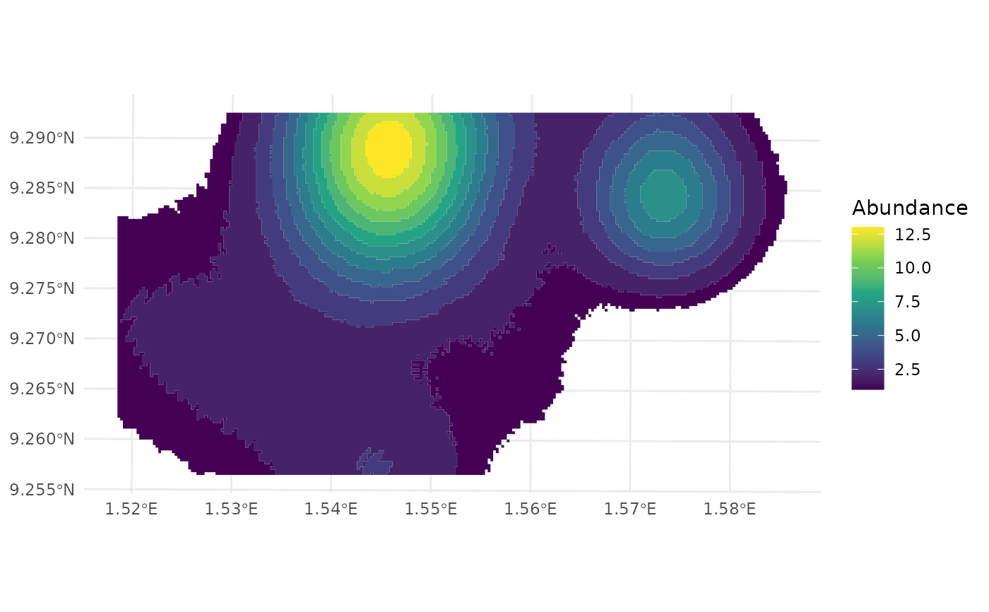
# Plot coverage raster
library(terra)
#> terra 1.9.27
terra::plot(spc$`Coverage raster`)


## Bandwidth estimate with uncertainty
spc$Bandwidth
#>    sigma       SE   CI_low  CI_high  n_sites isopleth 
#> 1225.784  164.128  799.379 1418.791   13.000    0.950 

## Coverage area summary
spc$`Coverage stats`
#> # A tibble: 1 × 5
#>   `Spatial coverage (km²)` `Bandwidth σ` `Bandwidth SE` `Detection sites (n)`
#>                      <dbl>         <dbl>          <dbl>                 <int>
#> 1                     33.9         1226.           164.                    13
#> # ℹ 1 more variable: `Isopleth level` <dbl>