Calculate observed spatial coverage of species

This function calculates the Observed Spatial Coverage of a species like Home Range, but based on camera trap data. The term home range is typically associated with dynamic movement data, such as those recorded by radio-tracking or GPS devices, which provide continuous or near-continuous tracking of an individual animal's movements. Since camera traps are static and only capture presence/absence or activity within their specific locations, the concept of home range might not fully apply.

Usage

mm_spatial_coverage(
  data,
  site_column,
  size_column = NULL,
  longitude,
  latitude,
  crs = c(4326, NULL),
  study_area = NULL,
  resolution,
  spread_factor = 0.1
)

Arguments

data

A data frame containing species occurrence records, including site, longitude, latitude, and optionally size (abundance).

site_column

Column name specifying the site identifier.

size_column

Optional column specifying the abundance of species at each site. Defaults to NULL, in which case counts per site are used.

longitude

Column name specifying the longitude of observation sites.

latitude

Column name specifying the latitude of observation sites.

crs

A vector of length two specifying the coordinate reference systems: c(crs1, crs2).

• crs1 represents the current CRS of the data (e.g., 4326 for latitude/longitude).

• crs2 represents the CRS to transform into (e.g., "EPSG:32631", a UTM EPSG code) for accurate distance calculations. If crs2 is NULL, no transformation is applied. Defaults to c(4326, NULL)

study_area

An optional simple feature (sf) polygon representing the study area. If provided, the raster extends to cover the area.

resolution

Numeric value specifying the spatial resolution (grid size) for rasterization.

spread_factor

A scale factor for the half-normal distribution. Higher values create a more spread-out distribution, while lower values make it more concentrated. The value must be in ]0; 1]

Value

A list containing:

• Coverage raster: A raster object representing species abundance across space.

• Coverage stats: A tibble with spatial coverage statistics, including area (km²), average abundance, maximum abundance, and standard deviation.

Details

The function applies a half-normal kernel to model species abundance over space, using the scale rate to control the spread of the distribution:

$$\bar{K}(x) = \frac{\sum w * \text{e}^{(-0.5 * (\frac{x}{\sigma})^2)}}{N}$$

where:

• \(\bar{K}(x)\) is the mean abundance kernel across all sites,

• \(w\) is the species abundance at each site,

• \(\sigma\) is the standard deviation of the spatial distance (scaled by spread_factor),

• \(N\) is the total number of sites.

Examples

library(dplyr)
cam_data <- system.file("penessoulou_season2.csv", package = "maimer") %>%
  read.csv() %>%
  dplyr::filter(Species == "Erythrocebus patas")

spc <- mm_spatial_coverage(
  data = cam_data,
  site_column = Camera,
  crs = "EPSG:32631", ,
  resolution = 30,
  spread_factor = 0.4,
  size_column = Count,
  longitude = Longitude,
  latitude = Latitude
)

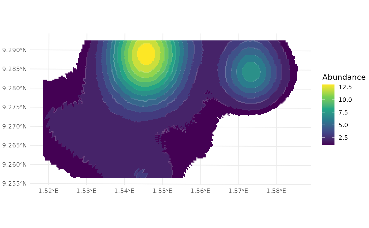
## Abundance stats
spc[[2]] %>%
  dplyr::select(-1)
#> # A tibble: 1 × 4
#>   `Spatial coverage (km²)` `Average abundance` `Maximum abundance`
#>                      <dbl>               <dbl>               <dbl>
#> 1                     22.6                   7                  13
#> # ℹ 1 more variable: `Standard Deviation` <dbl>

## Plot spatial coverage
library(ggplot2)
spc_vect <- terra::as.polygons(spc[[1]]) %>%
  sf::st_as_sf()

ggplot() +
  geom_sf(data = spc_vect, aes(fill = Abundance), color = NA) +
  theme_minimal() +
  scale_fill_viridis_c()