Calculate the temporal shift of one species' activity over two periods

This function estimates and analyzes the temporal shift in the activity of a species between two time periods using kernel density estimation. It computes the activity distributions and determines the magnitude and direction of the shift.

Usage

mm_temporal_shift(
  first_period,
  second_period,
  convert_time = FALSE,
  xscale = 24,
  xcenter = c("noon", "midnight"),
  n_grid = 128,
  kmax = 3,
  adjust = 1,
  width_at = 1/2,
  format = "%H:%M:%S",
  time_zone,
  plot = TRUE,
  linestyle_1 = list(),
  linestyle_2 = list(),
  posestyle_1 = list(),
  posestyle_2 = list(),
  ...
)

Arguments

first_period: A numeric vector representing activity times in radians for the first period.
second_period: A numeric vector representing activity times in radians for the second period.
convert_time: Logical. If TRUE, converts times to radians before analysis.
xscale: A numeric value to scale the x-axis. Default is 24 for representing time in hours.
xcenter: A string indicating the center of the x-axis. Options are "noon" (default) or "midnight".
n_grid: An integer specifying the number of grid points for density estimation. Default is 128.
kmax: An integer indicating the maximum number of modes allowed in the activity pattern. Default is 3.
adjust: A numeric value to adjust the bandwidth of the kernel density estimation. Default is 1.
width_at: Numeric. The fraction of maximum density at which the activity width is measured (default is 0.5).
format: Character. Format of time input (default is "%H:%M:%S"). Used if convert_time = TRUE.
time_zone: Character. Time zone for time conversion. Required if convert_time = TRUE.
plot: Logical. If TRUE, generates a plot comparing the activity distributions of the two periods.
linestyle_1: List. Line style settings for the first period's density plot. Includes linetype, linewidth, and color.
linestyle_2: List. Line style settings for the second period's density plot. Includes linetype, linewidth, and color.
posestyle_1: List. Marker style settings for the first period's density range. Includes shape, size, color, and alpha.
posestyle_2: List. Marker style settings for the second period's density range. Includes shape, size, color, and alpha.
...: Additional arguments (currently unused).

Value

A list containing:

A tibble with:

First period range: The start and end times of active periods in the first dataset.
Second period range: The start and end times of active periods in the second dataset.
Shift size (in hour): The absolute difference in activity duration between the two periods.
Move: A categorical description of the shift ("Forward", "Backward", "Expanded", "Contracted", etc.).

A plot (optional): A ggplot2 object visualizing the density distributions if plot = TRUE.

Examples

library(ggplot2)
# Using radians as input

first_period <- c(1.3, 2.3, 2.5, 5.2, 6.1, 2.3)  # Example timestamps for period 1
second_period <- c(1.8, 2.2, 2.5)  # Example timestamps for period 2
result <- mm_temporal_shift(first_period, second_period, plot = TRUE, xcenter = "noon",
                            linestyle_1 = list(color = "gray10", linetype = 1, linewidth = 1),
                            linestyle_2 = list(color = "#b70000", linetype = 5, linewidth = .5))

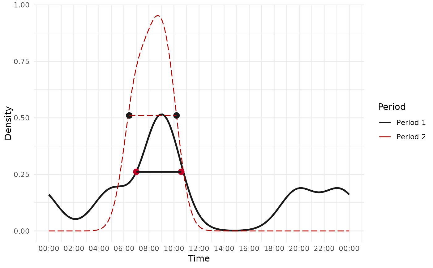result
#> [[1]]
#> # A tibble: 1 × 4
#>   `First period range` `Second period range` `Shift size (in hour)` Move    
#>   <chr>                <chr>                                  <dbl> <chr>   
#> 1 06:59:32 - 10:34:58  06:25:31 - 10:12:18                     0.19 Backward
#> 
#> $plot

#> 

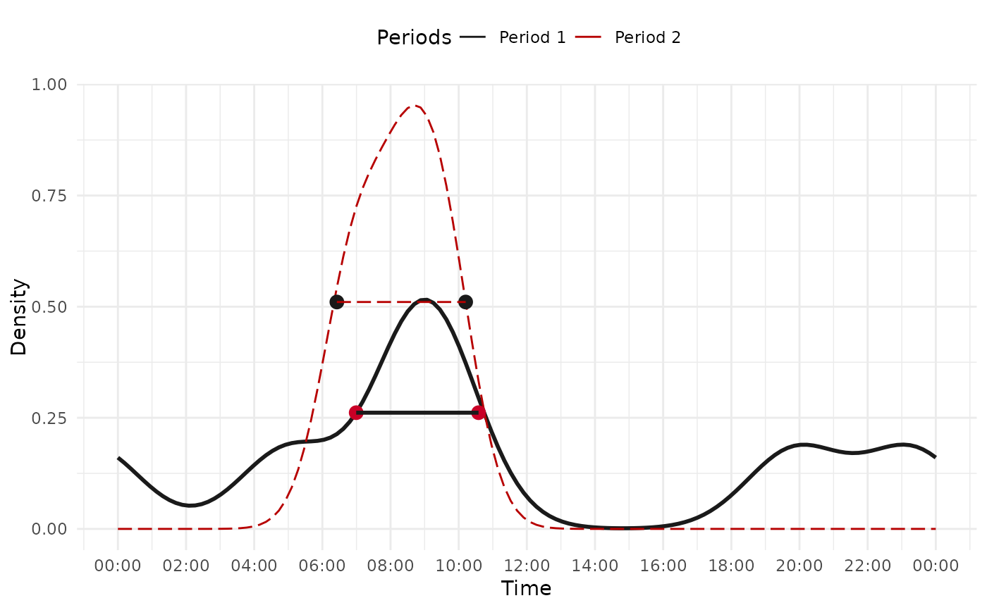
# customize the graph associated result
result$plot+
  labs(color = "Periods")+
  theme(legend.position = "top")


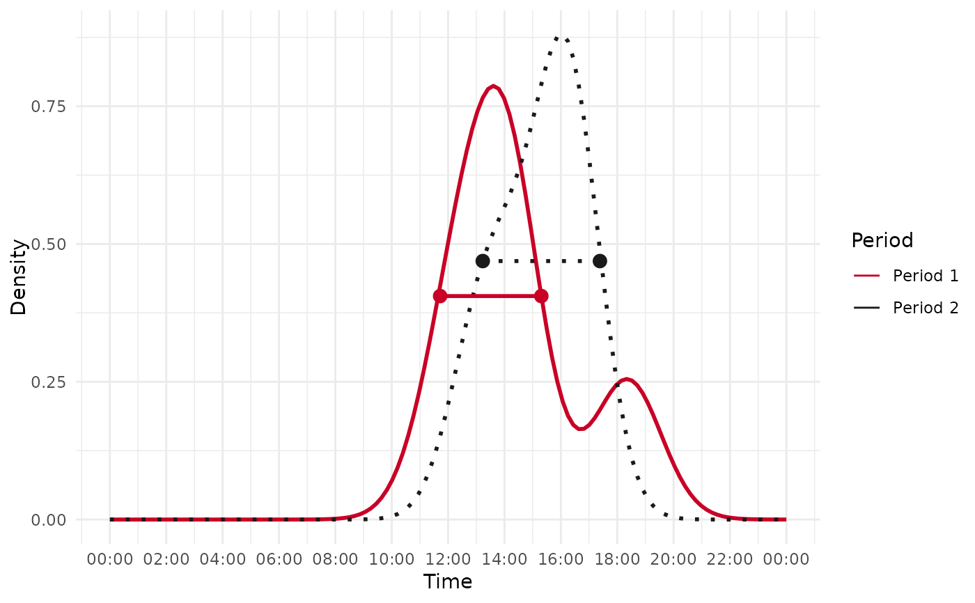
# Using time strings as input
first_period <- c("12:03:05", "13:10:09", "14:08:10", "14:18:30", "18:22:11")
second_period <- c("13:00:20", "14:20:10", "15:55:20", "16:03:01", "16:47:00")
result <- mm_temporal_shift(first_period, second_period,
                            convert_time = TRUE,
                            format = "%H:%M:%S",
                            time_zone = "UTC")