Distance Sampling with Camera Traps
Source:vignettes/articles/distance_sampling_guide.Rmd
distance_sampling_guide.RmdDistance Sampling with Camera Traps: A Comprehensive Guide
Introduction
Distance sampling represents a fundamental advance in wildlife population estimation, addressing one of ecology’s most persistent challenges: accounting for imperfect detection. Originally developed in the early 1990s for line and point transect surveys conducted by human observers, this method has recently been adapted for camera trap studies. The core innovation of distance sampling lies in its ability to correct density estimates by explicitly modeling how detection probability decreases with distance from the observer.
Traditional wildlife surveys face a limitation: not all animals present in a study area are observed. Animals farther from an observer or survey line are progressively more likely to be missed. Distance sampling confronts this issue directly by measuring the perpendicular distance between detected animals and survey points or lines, then using these measurements to estimate the probability of detection as a function of distance. This detection function allows us to extrapolate from observed animals to the total population, accounting for those individuals that were present but undetected.
From Human Observers to Camera Traps
Traditional Point Transect Surveys
In conventional point transect distance sampling, a human observer stands at a fixed location for a brief moment and records all animals detected within their field of view, along with the distance to each animal. The observer then moves to the next point, repeating this process across the study area. This approach assumes that detection probability is perfect at the point itself (distance zero) and decreases with increasing distance.
The Camera Trap Adaptation
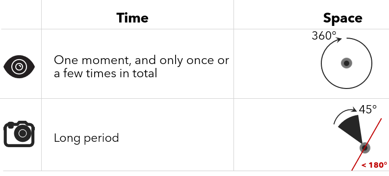
Camera traps share fundamental similarities with human point transect surveys. Both methods record animals from a fixed point in space, creating a snapshot of detections at specific moments. However, camera traps introduce important differences (see Figure 1) that required modification of the traditional distance sampling framework.
Where a human observer samples a point for mere seconds and typically visits only once or a few times, a camera trap samples continuously for days, weeks, or months. Human observers can pivot 360° around a point, whereas cameras remain fixed, sampling only a fraction of a circle determined by their viewshed angle (e.g 45°, less than 180°). These differences necessitated the incorporation of temporal and spatial effort components into the camera trap distance sampling model.
The Mathematical Framework
Basic Density Equation
The camera trap distance sampling model builds upon the traditional distance sampling equation but incorporates the unique characteristics of camera trap surveys. The fundamental equation for estimating density is:
D = N / (πw² × e × p̂)
In this equation, N represents the total number of detection events recorded across all cameras, w is the truncation distance beyond which detections are excluded from analysis, e quantifies the sampling effort (see section below for detail), and p̂ estimates the probability of detecting an animal within the truncation distance.
The truncation distance serves an important purpose. Beyond a certain distance, detection becomes highly uncertain and including these distant observations can introduce bias. We typically examine the distribution of detection distances and choose a truncation point that balances retaining sufficient data while excluding unreliable distant detections. The recommended truncation is 2-15m (Howe et al. 2017).
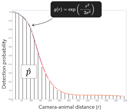
Concerning p̂, it is the total detection probability within the study area. As we will see later, it is the area under the curve of the detection function. \(\hat{p} = \int_{r_{min}}^{r_{max}} g(r)\, dr\), where \(r_{min}\) is the left truncation distance (minimum distance), and \(r_{max}\) is the right truncation distance (maximum distance).
Understanding Sampling Effort
Sampling effort for camera traps requires careful consideration of both temporal and spatial dimensions. A camera operating for longer periods accumulates more sampling effort, as does a camera with a wider field of view.
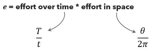
The effort equation captures this: \(e = \frac{\theta \times T}{2\pi \times t}\)
Here T represents the total time the camera was operational and actively sampling, θ denotes the camera’s viewshed angle in radians (the horizontal extent of its field of view), and t is a predetermined time interval at which animal-camera distances are measured. The denominator 2π represents a full circle, so the fraction θ/(2π) expresses what proportion of a complete circle the camera samples.
The time interval t deserves particular attention. For each detection event, researchers must measure the distance between camera and animal at regular intervals throughout the time animals remain visible. If animals move quickly or are rare, smaller intervals (0.25 to 3 seconds) provide more accurate distance measurements. This interval effectively determines how many “snapshots” are taken of each detection event.
The Detection Function
Central to distance sampling is the detection function, which models how detection probability declines with increasing distance from the camera. This function must satisfy a critical assumption: detection probability equals one at distance zero. In other words, an animal directly in front of the camera is always detected.
The detection function typically takes one of several mathematical forms, each characterized by a key function that describes the general shape of detection probability decline. The most commonly used key functions are the half-normal and hazard-rate models.
The Half-Normal Key Function
The half-normal key function assumes that detection probability decreases following a bell-curve shape (without the ascending portion). It contains a single scale parameter σ that determines how quickly detection probability falls off with distance. When detection probability drops relatively uniformly with distance, the half-normal often provides a good fit.
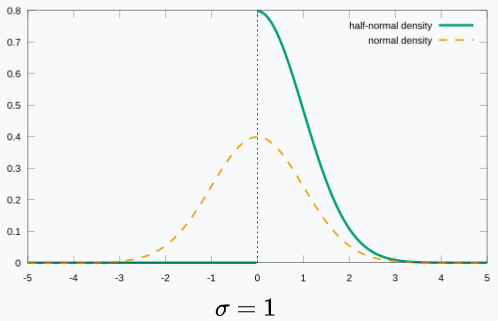
The half-normal key function is \(\exp\!\left(-\frac{r^{2}}{2\sigma^{2}}\right)\) where r is the camera-animal distances. Note that it is called Half-normal because it considers one part (here, the right-hand side) of a normal distribution. With this function, any negative distance leads to zero detection probability. At a distance close to zero, the probability is close to 1. As the distance increases, the detection probability decreases.
The Hazard-Rate Key Function
The hazard-rate key function offers more flexibility through both scale and shape parameters. This function can accommodate situations where detection probability remains relatively high across moderate distances before dropping more steeply at greater distances. The shape parameter controls this characteristic shoulder in the detection curve. The Hazard-rate key function is \(1- \exp\!\left(-(\frac{r}{\sigma^{2}})^{-b}\right)\). \(b\) is function-specific parameter.
The Uniform Key Function
Less commonly used, the uniform key function assumes constant detection probability across all distances up to the truncation point. This function serves primarily as a baseline and typically requires adjustment terms to provide realistic fits to data. The uniform key function is \(\frac{1}{w}\), with \(w\) the truncation distances.
Adjustment Terms
Real-world detection data rarely follows the smooth curves of theoretical key functions perfectly. Animals may be more or less detectable at certain distances due to vegetation structure, terrain, or behavior. Adjustment terms allow the detection function to flex and accommodate these departures from the idealized key function shape.
Three types of adjustment terms are available: cosine, Hermite polynomial, and simple polynomial. These mathematical functions add bumps and wiggles to the basic key function curve, improving the fit to observed data. Each adjustment term is characterized by its order, which determines the complexity of the added flexibility.
Cosine adjustments represent the most commonly used approach. When applied to half-normal or hazard-rate key functions, cosine adjustments of orders 2, 3, 4 and higher can be sequentially added. For a uniform key function, orders begin at 1. The adjustment terms are scaled by the truncation distance, ensuring they remain appropriately sized relative to the sampling range.
Hermite polynomial adjustments offer an alternative, though they restrict flexibility by allowing only even orders (2, 4, 6, and so on). Simple polynomial adjustments follow the same even-order restriction. The choice among adjustment types typically makes less difference than whether adjustments are included at all.
Model Selection Through AIC
When adjustment terms are considered, we face the question of how many to include. Too few adjustments may fail to capture important features of the detection process, while too many can lead to overfitting and implausible detection functions. The Akaike Information Criterion (AIC) provides a principled approach to this selection problem.
The AIC balances model fit against complexity, penalizing additional parameters. Distance sampling software typically implements a sequential forward selection procedure. It begins with a key function alone, calculates the AIC, then adds adjustment terms one at a time. If adding an adjustment improves (lowers) the AIC, it is retained. The process continues until adding further adjustments fails to improve the AIC, at which point the previous model is selected as optimal.
Ensuring Monotonicity
A fundamental biological reality dictates that detection probability cannot increase with distance from the camera. Yet when adjustment terms are added to detection functions, the resulting curve may develop unrealistic humps where detection probability rises at greater distances before falling again. Monotonicity constraints address this problem.
Two levels of monotonicity enforcement are possible. Weak monotonicity requires that detection probability at any distance be less than or equal to detection probability at distance zero. Strict monotonicity imposes a stronger requirement: detection probability must decrease (or at minimum remain constant) at each point compared to the previous shorter distance. Strict monotonicity represents the more biologically realistic assumption and is typically applied by default when fitting models without covariates.
These constraints operate during model fitting by evaluating detection probability at regularly spaced points across the distance range. If the constraints are violated, the optimization algorithm adjusts parameters to satisfy them. However, monotonicity constraints cannot be enforced when covariates are included in the model, as detection probability may legitimately vary in complex ways across different covariate values.
Accounting for Animal Activity Patterns
The Activity Level Correction
Many species exhibit predictable periods of inactivity when they are unavailable for detection. Nocturnal species rest during daylight hours, while diurnal species are inactive at night. Some species have regular midday rest periods even during their active season. If camera data includes these inactive periods, density estimates require correction.
The correction factor is conceptually straightforward. If animals are active and available for detection only a proportion a of the day, the raw density estimate D overestimates true density by a factor of 1/a. The corrected density estimate becomes: \(D{c} = D \times \frac{1}{a}\)
Determining activity level a requires careful analysis of detection timing patterns. The proportion of time animals are active is calculated from the temporal distribution of detection events across the full 24-hour cycle. This analysis assumes that when animals are active, they are equally likely to be detected at any time during the active period.
Practical Analysis Workflow
We provided here full analysis workflow to apply distance sampling to estimate animal density using ct R package.