Plot a calendar heatmap of daily camera trap activity

Visualises a year of camera-trap records as a calendar heatmap. Tiles are shaded by the number of records per day, or by the summed value of a chosen column. A count distribution can optionally be fitted to the daily values and used for the shading.

Usage

ct_plot_calendar(
  data,
  datetime,
  format = NULL,
  size_column = NULL,
  only_month = NULL,
  fit_distribution = FALSE,
  abbreviate_month_name = FALSE,
  month_name = NULL,
  day_name = NULL,
  number_of_column = 4,
  low = NULL,
  high = NULL,
  palette = NULL,
  na_value = "grey95",
  show_day_number = TRUE,
  title = NULL
)

Arguments

data: A data frame of records, one row per detection.
datetime: Column holding the date or date-time of each record.
format: Optional date format(s) passed to as.Date() via tryFormats. If NULL (default), a set of common date and date-time formats is tried.
size_column: Optional column whose values are summed per day, for example the number of individuals recorded in each detection. If omitted, the number of records (detections) per day is used instead.
only_month: Optional integer vector of month numbers (1 to 12) to keep, for example 3:5. Records outside these months are dropped and only those month panels are drawn. Default NULL (the whole year).
fit_distribution: Logical. If TRUE, a count distribution is fitted to the records per day over the displayed period (days with no record count as zeros) with ct_fit_distribution(), and the fitted distribution is reported in the plot subtitle. Tiles are then shaded by the fitted density, that is the probability of each day's count under the model. The calendar therefore becomes a typicality map, not an activity map: the brightest tiles are the most probable days under the fitted distribution, which for zero-heavy camera-trap data are usually the days with no detection, while busier days carry rarer counts and appear darker. See Details. Default FALSE.
abbreviate_month_name: Logical. Use three-letter month names. Ignored when month_name is supplied. Default FALSE.
month_name: Optional length-12 character vector of month labels, for localisation. Defaults to the English month names.
day_name: Optional length-7 character vector of weekday labels, Monday first. Defaults to c("Mon", "Tue", "Wed", "Thu", "Fri", "Sat", "Sun").
number_of_column: Number of month panels per row. Default 4.
low, high: Optional start and end colours for a two-colour gradient fill. When both are supplied they override palette.
palette: Optional fill palette. Either a single viridis option letter (for example "C"), or a vector of two or more colours for a custom gradient. Default NULL (viridis option C).
na_value: Fill colour for days with no records. Default "grey95".
show_day_number: Logical. Print the day number inside each tile. Default TRUE.
title: Optional plot title. Generated automatically when NULL.

Value

A ggplot2::ggplot object.

Details

With fit_distribution = FALSE the calendar is an activity map: tiles are shaded by the records per day (or the summed size_column), so busier days are brighter.

With fit_distribution = TRUE the calendar is instead a typicality map. A single distribution is fitted to the whole displayed period, and each tile is shaded by the fitted probability of that day's count. Because most days have no detection, the count of zero is the most probable value, so empty days receive the highest density and the brightest colour, while the rarer busy days appear darker. The map highlights how typical or unusual each day is under the model, rather than how much activity occurred. Use fit_distribution = FALSE if you want activity intensity instead.

Examples

library(dplyr)
data(ACBR)

# The calendar covers one year at a time, so keep a single year.
d2024 <- ACBR$acbr_data %>%
  # Filter to independent (10min separated) detections
  ct_independence(species_column = species,
                  datetime = datetime,
                  format = "%Y-%m-%d %H:%M:%S",
                  threshold = 10*60
  ) %>%
  # Select data for 2025 year
  filter(lubridate::year(datetime) == 2025)

ct_plot_calendar(d2024, datetime = datetime,
                 size_column = count,
                 low = "gray", high = "red"
)

#'
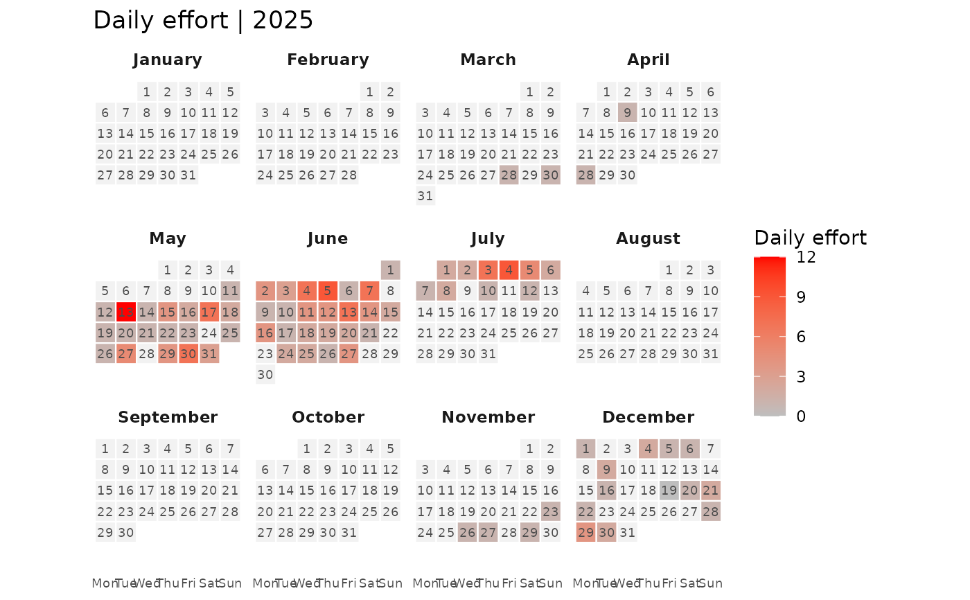