Extent of occurrence and area of occupancy (IUCN criterion B) • redlist

library(redlist)

Why criterion B

IUCN criterion B assesses a species’ geographic range through two metrics:

Extent of occurrence (EOO), the area of the smallest convex polygon that encloses all known sites of occurrence (section 4.9 of the Red List guidelines).
Area of occupancy (AOO), the total area of occupied cells on a 2 by 2 km reference grid (section 4.10, equation 4.1).

Both metrics need a clean set of occurrence records. In a full workflow those records come from rl_occurrences(), which returns an sf POINT object after resolving the IUCN name against the GBIF backbone and querying under all synonyms. rl_eoo() and rl_aoo() take that object directly. They also accept a plain data frame with longitude and latitude columns, which is what we use here so the vignette stays self contained.

occ <- data.frame(
  longitude = c(2.10, 2.62, 3.01, 2.44, 2.90, 1.83, 2.25, 3.14, 1.97, 2.71),
  latitude = c(9.12, 9.53, 9.04, 9.81, 9.33, 9.62, 10.10, 9.45, 9.90, 9.20)
)
head(occ)
#>   longitude latitude
#> 1      2.10     9.12
#> 2      2.62     9.53
#> 3      3.01     9.04
#> 4      2.44     9.81
#> 5      2.90     9.33
#> 6      1.83     9.62

Extent of occurrence

rl_eoo() projects the coordinates to a local equal area system, builds the convex hull, and returns its area in square kilometres along with the criterion B1 threshold the value reaches.

rl_eoo(occ)
#> Simple feature collection with 1 feature and 6 fields
#> Geometry type: POLYGON
#> Dimension:     XY
#> Bounding box:  xmin: 1.83 ymin: 9.04 xmax: 3.14 ymax: 10.1
#> Geodetic CRS:  WGS 84
#>   metric area_km2 n_records n_unique      method category_b1
#> 1    EOO 10586.91        10       10 convex hull          VU
#>                         geometry
#> 1 POLYGON ((3.01 9.04, 2.1 9....

The category_b1 column reports the most threatened band the area reaches ("CR", "EN" or "VU"), or NA when it meets none. This is the spatial threshold only. A full listing under criterion B also requires at least two of the subconditions (a) severe fragmentation or few locations, (b) continuing decline, and (c) extreme fluctuation.

The extent of occurrence is undefined with fewer than three unique locations, since no polygon can be drawn. In that case area_km2 is NA and a warning is issued.

rl_eoo(data.frame(longitude = c(2.1, 2.6), latitude = c(9.1, 9.5)))
#> Warning: EOO needs at least 3 unique locations, but 2 were found.
#> ℹ The extent of occurrence is undefined and reported as "NA".
#> Simple feature collection with 1 feature and 6 fields (with 1 geometry empty)
#> Geometry type: POLYGON
#> Dimension:     XY
#> Bounding box:  xmin: NA ymin: NA xmax: NA ymax: NA
#> Geodetic CRS:  WGS 84
#>   metric area_km2 n_records n_unique      method category_b1      geometry
#> 1    EOO       NA         2        2 convex hull        <NA> POLYGON EMPTY

Area of occupancy

rl_aoo() counts the occupied cells of a 2 by 2 km grid (each cell covering 4 square kilometres) and multiplies by the cell area.

rl_aoo(occ)
#> Simple feature collection with 1 feature and 6 fields
#> Geometry type: MULTIPOLYGON
#> Dimension:     XY
#> Bounding box:  xmin: 1.822794 ymin: 9.039459 xmax: 3.15264 ymax: 10.10663
#> Geodetic CRS:  WGS 84
#>   metric area_km2 n_records n_occupied_cells cell_size_km category_b2
#> 1    AOO       40        10               10            2          EN
#>                         geometry
#> 1 MULTIPOLYGON (((2.096724 9....

category_b2 reports the criterion B2 band in the same way as category_b1 above. Keep the default cell_size = 2000, since the criterion B2 thresholds assume the 2 by 2 km reference scale. Estimating AOO at a finer or coarser scale gives values that cannot be compared against those thresholds.

Working with an sf object

When you already have an sf POINT object, pass it straight in. Any coordinate reference system is accepted; geographic coordinates are reprojected to an equal area system before measurement.

pts <- sf::st_as_sf(occ, coords = c("longitude", "latitude"), crs = 4326)
rl_aoo(pts)
#> Simple feature collection with 1 feature and 6 fields
#> Geometry type: MULTIPOLYGON
#> Dimension:     XY
#> Bounding box:  xmin: 1.822794 ymin: 9.039459 xmax: 3.15264 ymax: 10.10663
#> Geodetic CRS:  WGS 84
#>   metric area_km2 n_records n_occupied_cells cell_size_km category_b2
#> 1    AOO       40        10               10            2          EN
#>                         geometry
#> 1 MULTIPOLYGON (((2.096724 9....

Mapping the polygons

Both functions return an sf object, so the geometry column carries the polygon behind each metric: the convex hull for EOO, and the occupied 2 km cells for AOO. Both come back in the input coordinate system, ready to plot or to write to a spatial file.

eoo_poly <- rl_eoo(occ)
aoo_poly <- rl_aoo(occ)
pts <- sf::st_as_sf(occ, coords = c("longitude", "latitude"), crs = 4326)

plot(sf::st_geometry(eoo_poly), border = "steelblue", lwd = 2,
     main = "EOO hull and AOO cells")
plot(sf::st_geometry(aoo_poly), col = "#f4a58255", border = "tomato", add = TRUE)
plot(sf::st_geometry(pts), pch = 20, add = TRUE)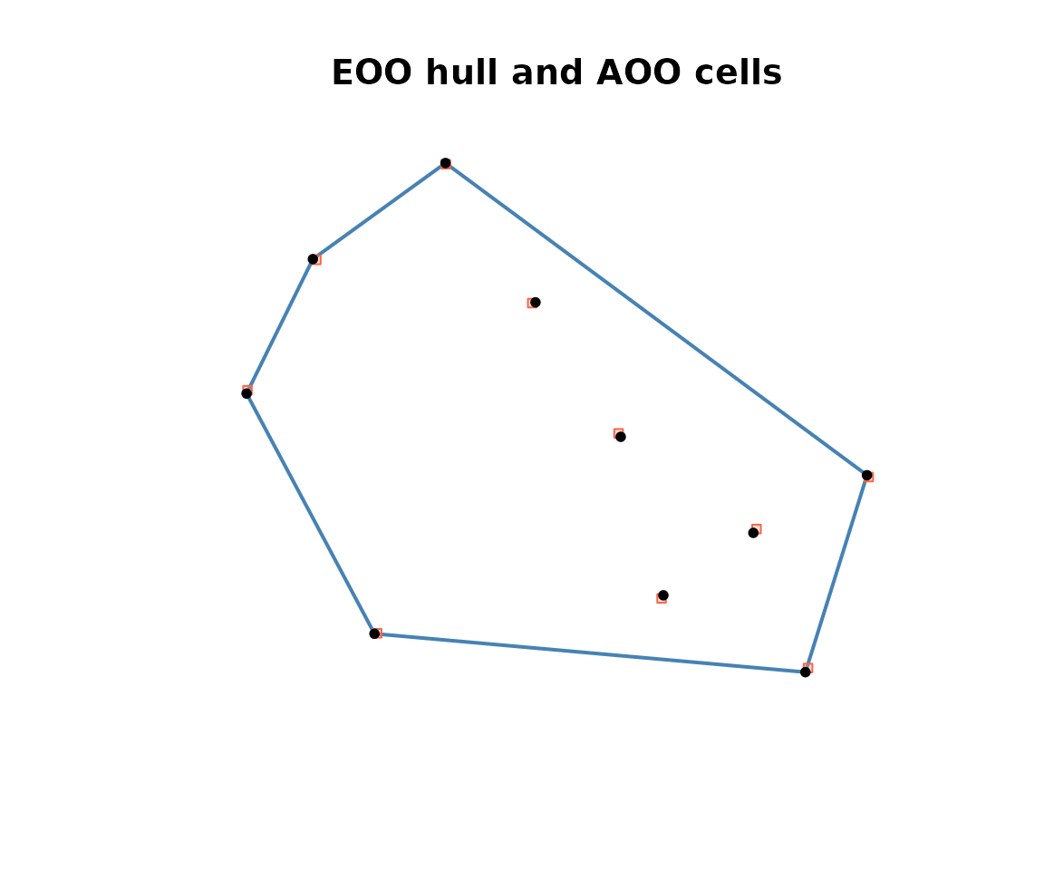

You can save either polygon with sf::st_write(), for example sf::st_write(eoo_poly, "eoo.gpkg").

Consistency between the two metrics

By definition AOO sits inside EOO, so EOO should never be smaller than AOO. When a sparse convex hull makes EOO come out below AOO, the guidelines recommend raising EOO to equal AOO. rl_eoo() and rl_aoo() report each metric on its own; combine them and apply that adjustment when you compile the assessment.

eoo <- rl_eoo(occ)
aoo <- rl_aoo(occ)
data.frame(
  metric = c("EOO", "AOO"),
  area_km2 = c(eoo$area_km2, aoo$area_km2),
  category = c(eoo$category_b1, aoo$category_b2)
)
#>   metric area_km2 category
#> 1    EOO 10586.91       VU
#> 2    AOO    40.00       EN